Concept Whitening for Explainable AI in Computer Vision
What is Whitening? How Concept Whitening can alter existing ML models to become better self-explainable
Recently, Chen, Z., Bei, Y. and Rudin, C. at Duke University proposed a new technique called Concept Whitening (CW)
- Why Explainable AI?
- Limitations of post-hoc explanations
- Alternatives to post-hoc approaches
- What is Whitening?
- Concept Whitening
- Conclusion
1. Why Explainable AI?
First off, why we need Explainable AI in the first place?
Most of the time, correct predictions only partially solve the problem.
- Humans need explaination to build trust:
- Doctor can not just say that a patient is having cancer without any explanation.
- Business department need the reason why they have to make some decisions. They dont want to risk lots of money on something they don't even know.
- Improve the model performance as well as control the model's behavior such as bias, racism.
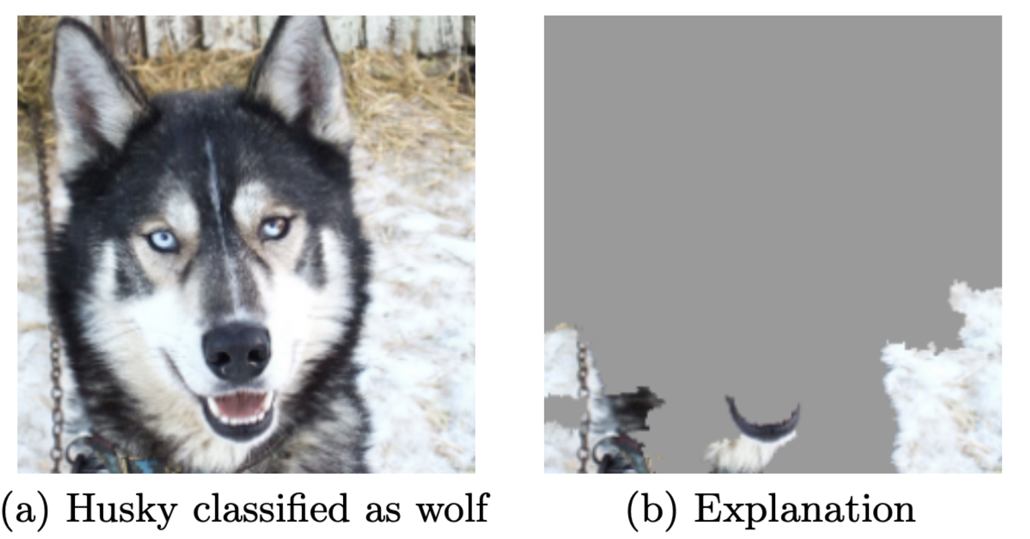 The model confused the husky to wolf because of the snow backgound behind. Picture Source
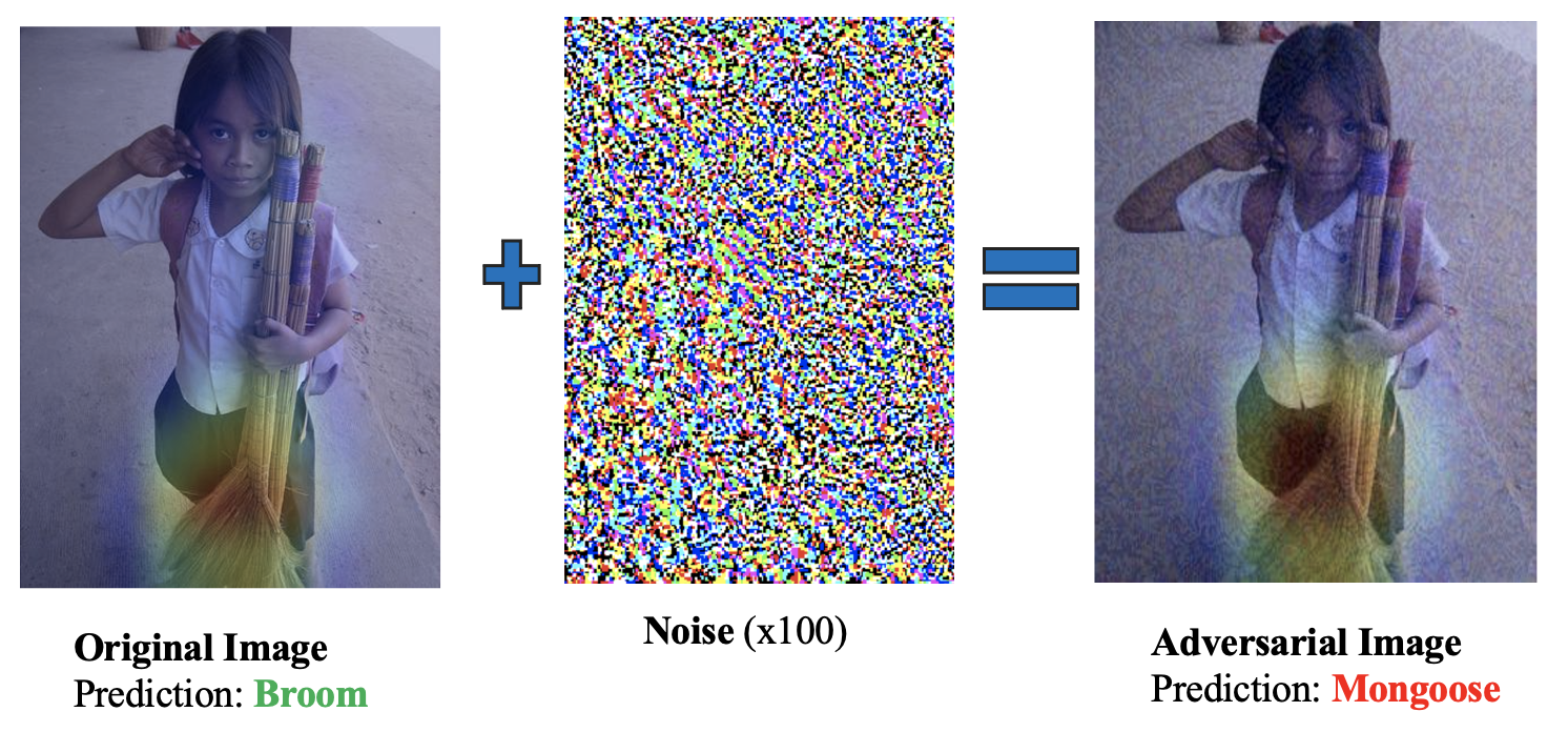
 - Avoid attacks like Adversarial attacks which use counterfactual examples to deceive the model.
2. Limitations of post-hoc explanations
There are two main categories in XAI: post-hoc explanation models and self-explainable models. For the former, we train a Machine Learning model first, then try to use another model to explain it later on. The latter approach aims to create self-explanatory models.
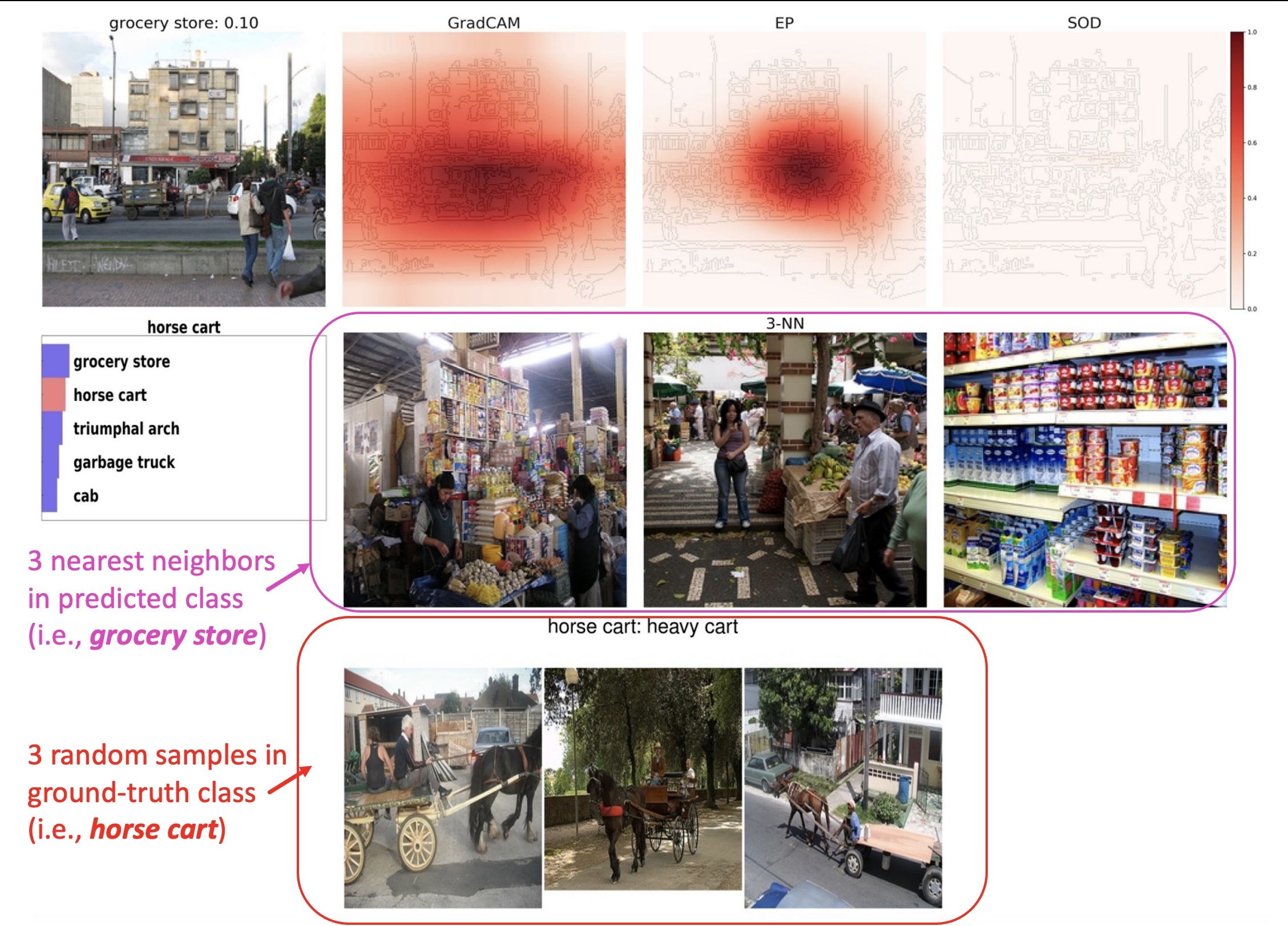
Post-hoc explanations focus on explaining the result of the model rather than how the model came up with the result. Let’s take Attribution (Saliency-based) method — a well-used approach in post-hoc explanations for neural networks — as an example. This approach highlights some important pixels of the image to indicate what the model paid attention to. However, it’s likely to highlight the edges of the objects, regardless of the class.
In recent work, Nguyen, G., Kim, D. and Nguyen, A. argue that attribution methods do not
help, but instead reduce the performance of human-AI teams compared to using only AI
3. Alternatives to post-hoc approaches
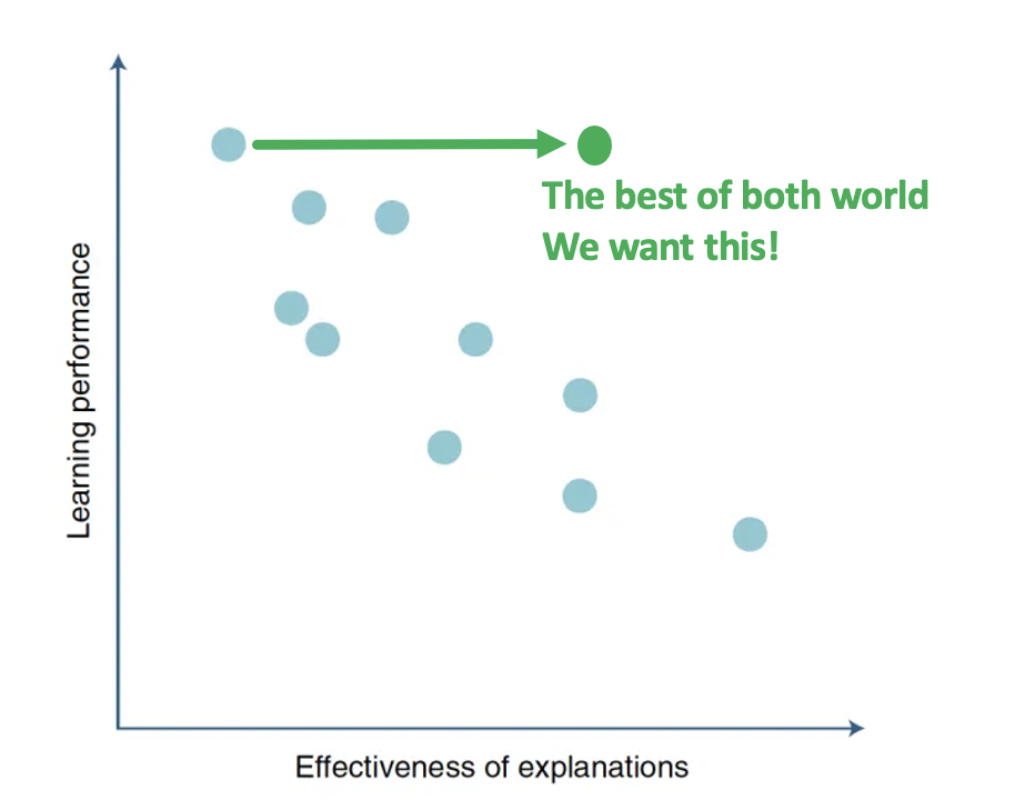
In general, there is a trade-off between performance and explainability: Black box models like deep neural networks gain high accuracy but get into trouble when it comes to explaining their results; More explainable models such as decision tree can be easier to understand, but the accuracy is not desirable, especially when the inputs consist of many dimensions like images.
Instead of creating a post-hoc explanation for black box models, an alternative is to create a model that is high-performance and self-explanatory. This can be archived by:
- A new architecture that is high-performance and self-explanatory. For example, Neural Backed Decision Trees
can match neural network accuracy while preserving the interpretability of a decision tree. - A method to alter existing high-performance models to become more transparent. Concept Whitening (CW)
belongs to this category.
We will get into Whitening and CW in the rest of this post.
4. What is Whitening?
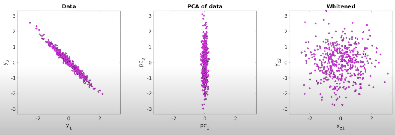
Whitening is a linear transformation process that transforms a set of random variables into a set of new random variables with identity covariance. Intuitively, whitening shrinks large data directions and expands small data directions.
Mathematically, given a random vector \(\mathbf{X}\) with a covariance matrix \(\mathbf{\Sigma}\), if the data points in \(\mathbf{X}\) are correlated, then the covariance \(\mathbf{\Sigma}\) will not be a diagonal matrix. Our aim is to decorrelate the covariance \(\mathbf{\Sigma}\), so that it will be a diagonal matrix. The covariance matrix is symmetric, thus it can be decomposed to \(\boldsymbol{U}^{\top} \boldsymbol{\Sigma} \boldsymbol{U}=\boldsymbol{\Lambda}\), where \(\boldsymbol{U}\) is the eigenvector matrix, and \(\boldsymbol{\Lambda}\) is the eigenvalue matrix. If we make the eigenvalues in \(\boldsymbol{\Lambda}\) all the same, then it would be the whitening process. This can be archived by normalizing \(\boldsymbol{\Lambda}\) to \(\boldsymbol{\Lambda}^{-1/2}\) at both sides: \(\mathbf{\Lambda}^{-1 / 2} \boldsymbol{\Lambda} \mathbf{\Lambda}^{-1 / 2}=\mathbf{I}\). Thus, we can pick a matrix \(\mathbf{W}=\mathbf{\Lambda}^{-1 / 2} \mathbf{U}^{\top}\), then project the original data \(\mathbf{X}\) onto \(\mathbf{W}\) to get new dataset \(\mathbf{Y}=\mathbf{W} \mathbf{X}\). We can observe that covariance matrix of the new dataset is an identity matrix:
\begin{equation}
\label{eqn:eq1}
\begin{split}
\mathbf{cov}(\mathbf{Y}) &= \mathbf{cov}(\mathbf{WX})
&= \mathbf{W} \mathbf{cov}(\mathbf{X}) \mathbf{W^{\top}}
&= \mathbf{\Lambda}^{-1 / 2} \mathbf{U}^{\top} \boldsymbol{\Sigma} \mathbf{U} {\mathbf{\Lambda}^{-1 / 2}}^{\top}
&= \mathbf{I}
\end{split}
\end{equation}
From Equation \ref{eqn:eq1} above, we can rewrite to get \(\mathbf{W^{\top}} \mathbf{W}\).
\[\mathbf{W} \mathbf{\Sigma} \mathbf{W}^{\top} =\mathbf{I}\] \[\mathbf{W} \mathbf{\Sigma} \mathbf{W}^{\top} \mathbf{W} = \mathbf{W}\] \[\mathbf{W}^{\top} \mathbf{W} =\mathbf{\Sigma}^{-1}\]Thus, the whitening transformation \(\mathbf{W}\) is the one that satisfies \(\mathbf{W}^{\top} \mathbf{W}= \mathbf{\Sigma} ^{-1}\). However, such matrix \(\mathbf{W}\) is not unique as whitening is rotation free. In particular, if \(\mathbf{W}\) is a whitening transform, so is any of its rotation \(\mathbf{W} \mathbf{Q}\) with \(\mathbf{Q}\) satisfies \(\mathbf{Q}^{\top} \mathbf{Q}=\mathbf{I}\).
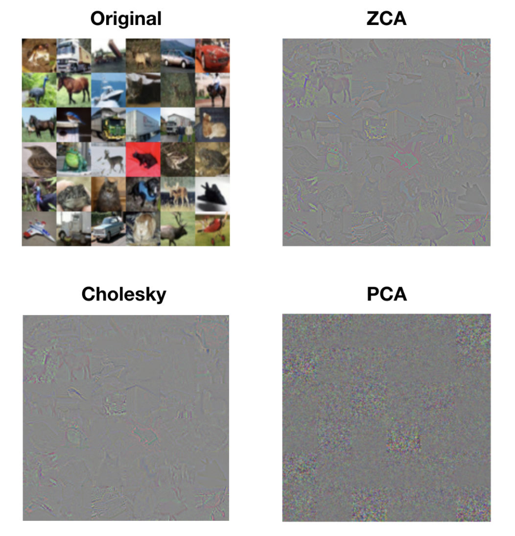
Depending on the choice of \(\mathbf{W}\), we have some common whitening methods such as ZCA whitening, PCA whitening, and Cholesky whitening. Figure below illustrates these techniques for image processing.
Concept Whitening uses ZCA whitening, first introduced as zero-phase component analysis, in the CW module as ZCA-whitened images still resemble normal images. ZCA whitening first transforms original data \(\mathbf{X}\) into the eigenbasis through shifting and rotating, scales it to normalize each dimension, then performs another rotation to get the desired basis. Figure below shows the ZCA whitening process on 2-dimensional inputs.
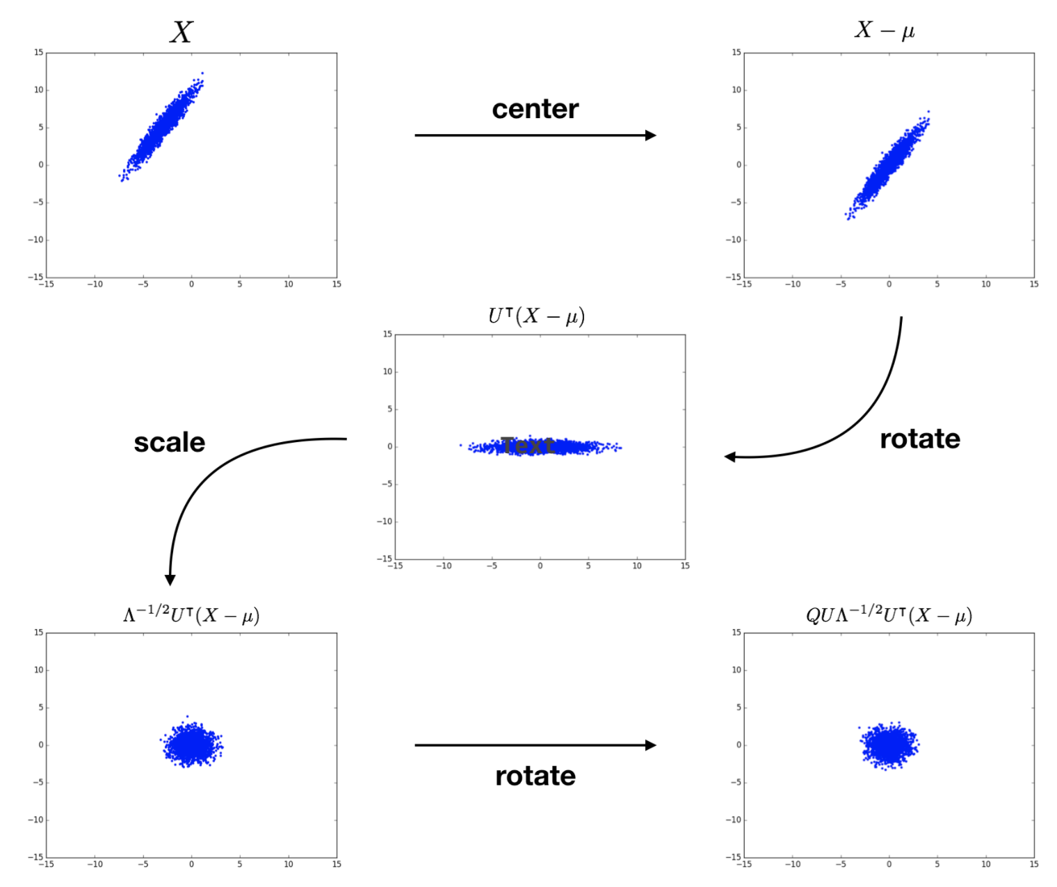
The ZCA whitening is defined as follows.
\[\mathbf{W}_{\mathrm{ZCA}}=\mathbf{U} \mathbf{\Lambda}^{-1 / 2} \mathbf{U}^{\top}= \mathbf{\Sigma}^{-1/2}\]5. Concept Whitening
Firstly, it’s worth having a look at the demo video of Concept Whitening (CW) from the authors to get a sense of it.
5.1. Ideas of CW
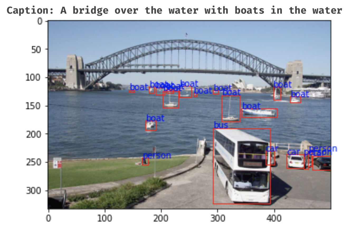
What is a concept? For an input image, it may contain many objects. Basically, concept is a thing (object instances like cats, dogs, cars, person), or stuff (e.g., sky, water) in the image. For example, concept can be plane, boat, person, or sky. It can be anything depending on how we define a concept.
CW is a module utilizing the Whitening transformation in neural network context and can replace BatchNorm layer
In addition to normalization effects as BatchNorm’s, CW decorrelates the CNN’s latent space and aligns the axes of the latent space along with the concepts through training to generate interpretable models.
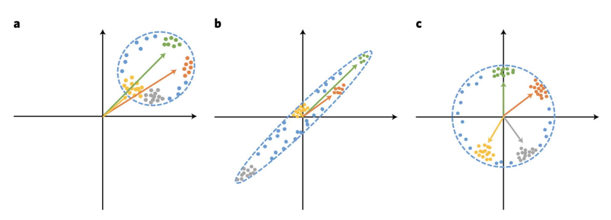
CW can represent the contributions of each concept to build intuition on how the model learns. Figure below demonstrates three possible data distributions in the latent space. CW (Fig. c) can help to disentangle the latent vectors so that they can be valid to represent the concepts.
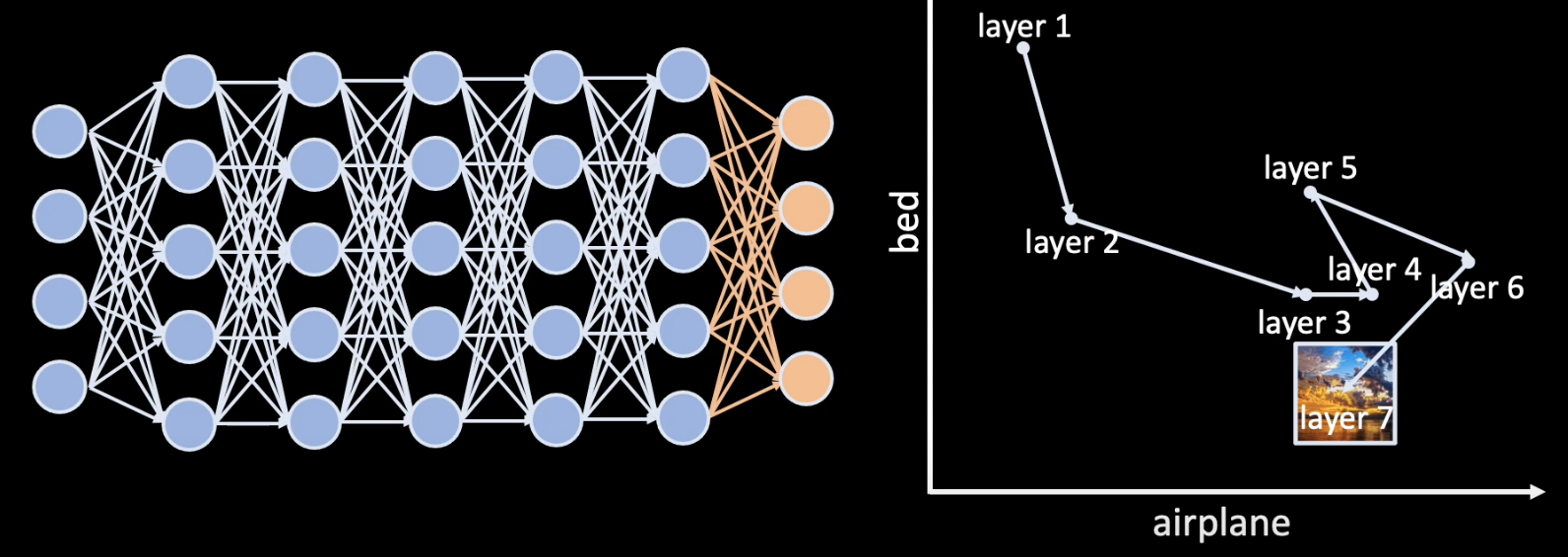
The trajectory of a sample in the space of concepts over different layers in the network can reveal how the model makes that decision throughout the training process.
5.2. How CW works
For standard settings, from input $x$, we will map $x$ to latent feature $z=\phi(x)$, and then make a prediction $y=g(z)$.
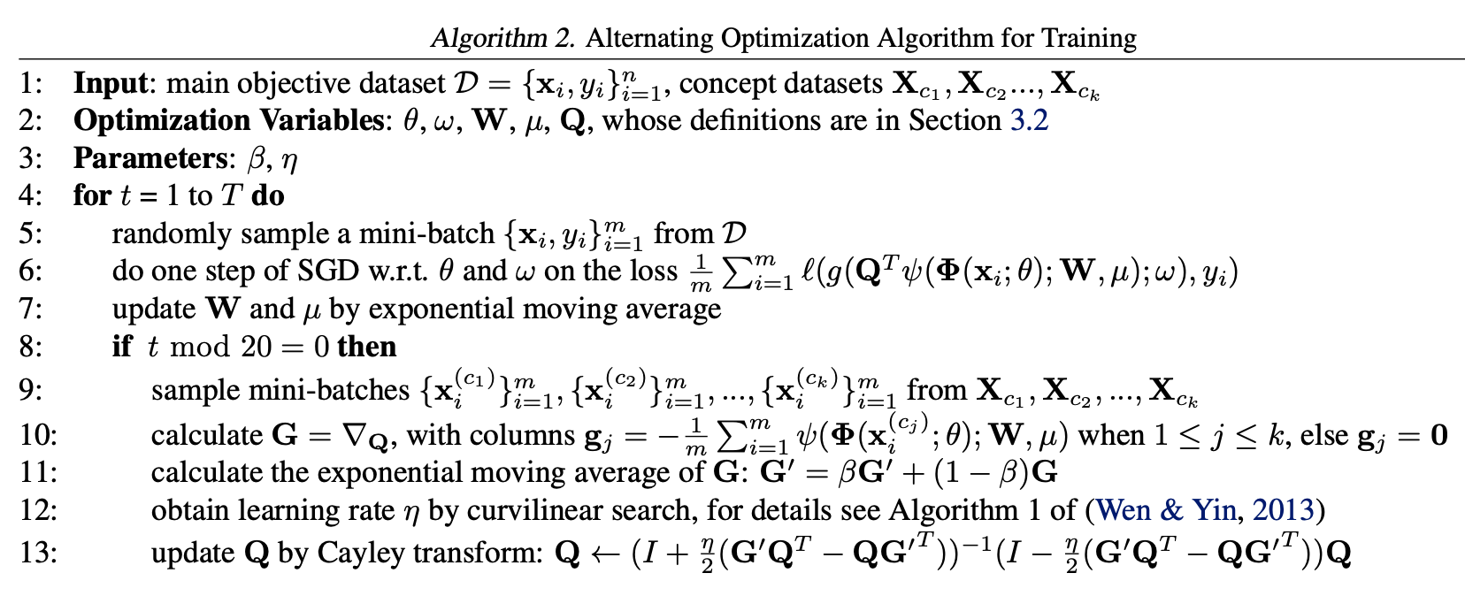
In the CW’s setting, besides minimizing the loss from $g$, we also optimize $\phi$ simultaneously with $g$ so that $z$ aligns with the desired concept.
Given $c_j$, $j=1$ to $k$, are the $k$ concepts that we are interested in. We have two sets of datasets: The concept dataset $X$ in which $X_{c_{j}}$ denotes a set of samples that activate the most in the concept $c_j$, and $n_j$ is the number of samples in $X_{c_{j}}$; The standard datasets $D$ — the images for classification task.
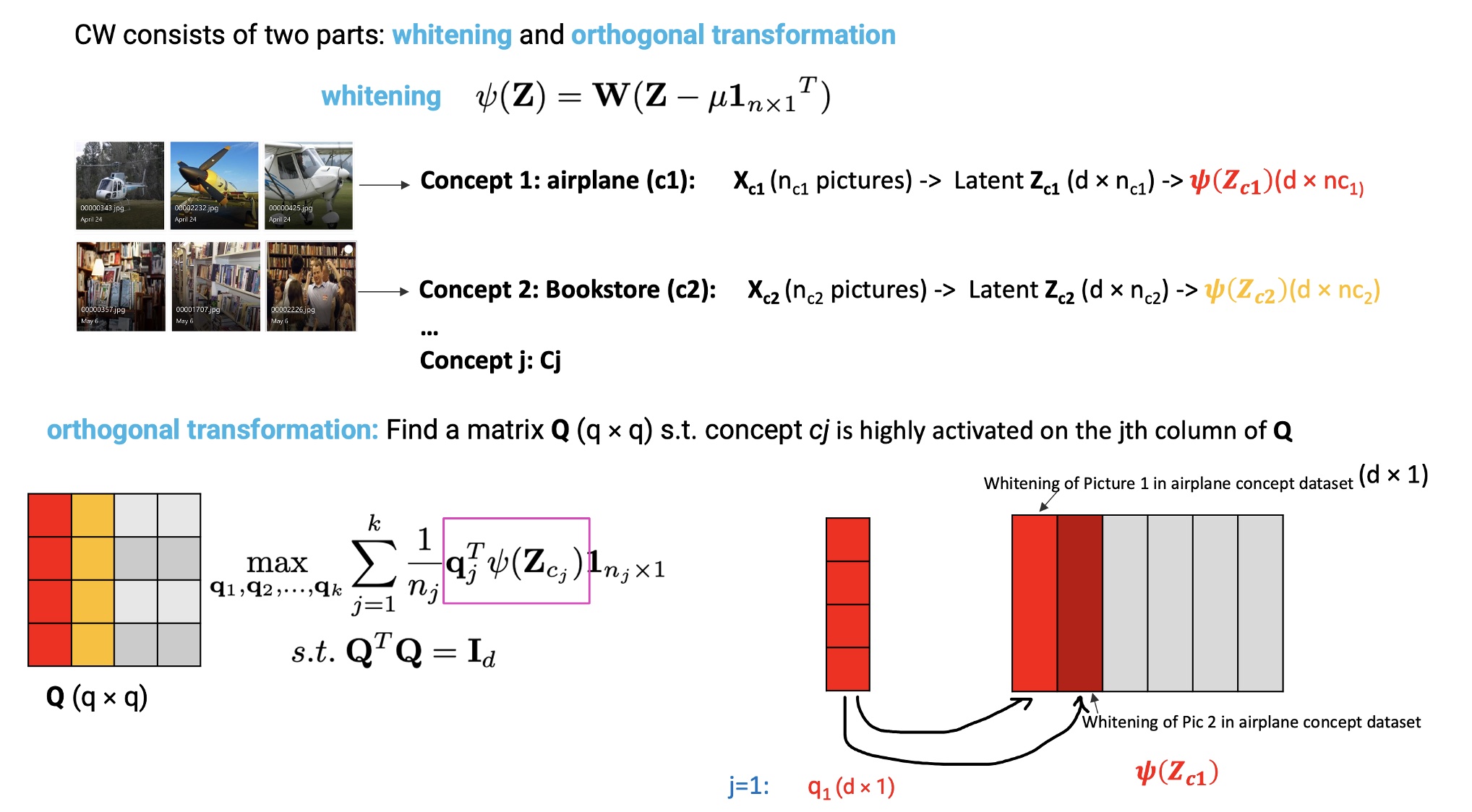
CW consists of two parts: whitening and orthogonal transformation. First, from $X_{c_{j}}$ (i.e., $n_j$ samples that activate the most in concept $c_j$), we get its latent representation matrix $Z_{c_{j}}$ ($d \times n_j$) in which each $d$-dimensional column contains the latent features of the $i$th sample of $X_{c_{j}}$. From the ZCA whitening, we need to find a rotation matrix $\mathbf{Q}$ ($d \times d$) to activate the data $X_{c_{j}}$ in $c_{j}$ concept. So, column $q_j$ of $Q$ is the $j$th axis. Specifically, we need to optimize the following objective:
\[\begin{array}{c} \max _{\mathbf{q}_{1}, \mathbf{q}_{2}, \ldots, \mathbf{q}_{k}} \sum_{j=1}^{k} \frac{1}{n_{j}} \mathbf{q}_{j}^{\top} \psi\left(\mathbf{Z}_{c_{j}}\right) \mathbf{1}_{n_{j} \times 1} \\ \text { s.t. } \mathbf{Q}^{\top} \mathbf{Q}=\mathbf{I}_{d} \end{array}\]where $\mathbf{\psi}$ is a whitening transformation parameterized by sample mean $\mathbf{\mu}$ and whitening matrix $\mathbf{W}$.
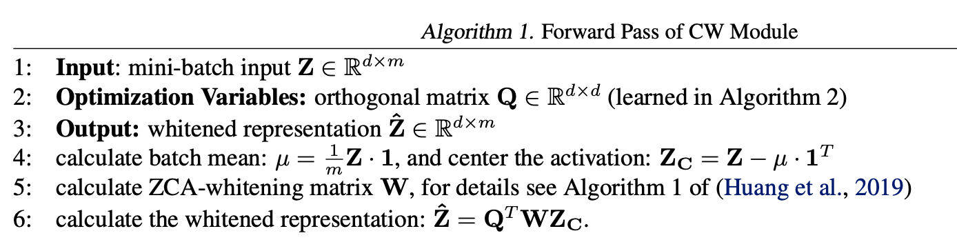
Thus, for mini-batch input \(\mathbf{Z} \in \mathbb{R}^{d \times m}\), the whitened representation $\mathbf{ \hat{Z} }= \mathbf{Q^{\top}} \mathbf{W} (\mathbf{Z}-\mu \cdot \mathbf{1}^{\top }) $ will be the same dimension as $\mathbf{Z}$.
5.3. Datasets
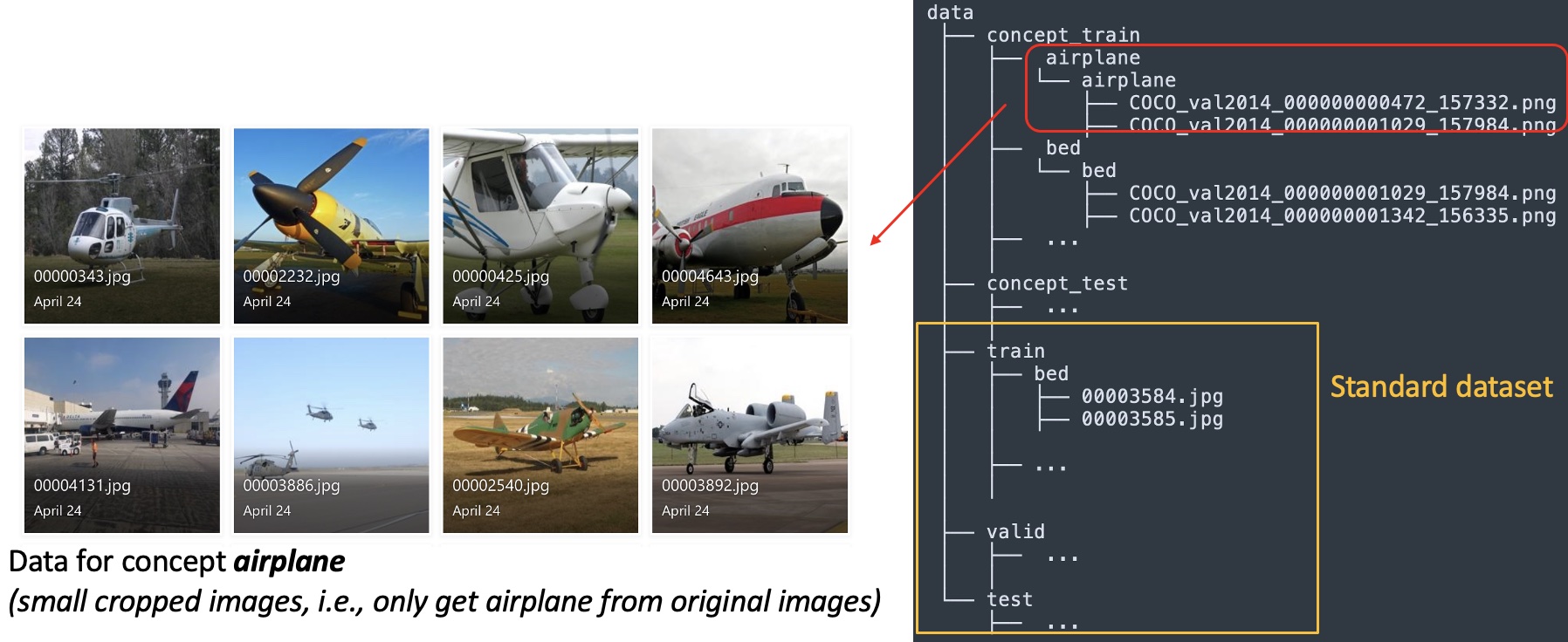
In the CW paper, the authors use Places365, a public dataset that well-used in training CNNs. In addition to images for classification, we need MS COCO dataset which contains concept images to train the CW module. Specifically, for each image in the data, a part of the image whose label and caption contain the concept will be cropped. For example, concept airplane is generated from image whose caption contains the word airplane and its label also is airplane. Figure below illustrates one example of the dataset.
5.4. Use case with ResNet18
CW can be used with any existing CNN models. For example, we can replace the second BatchNorm at the end of layer four of ResNet18
Dimensions after going through the CW module: Each input image is resized to $224\times224$, then is fed into a modified ResNet18 (with the CW module). The image goes through eight skip connects in which five will resize the image to a half. In that sense, each dimension of the image will be reduced from $224$ to $224 / 2^5 = 7$. So, each image would have a size of $7\times7$. The output after going through the CW module would be $7\times7\times512$, where 512 indicates the number of channels.
Orthogonality check: We use concept images from concept_test folder as the inputs. For each input, we know which concept it belongs to. We feed the inputs through the network to get $7\times7\times512$ output vectors as discussed above. Then, we flatten these vectors into 1D vectors (i.e., $25088$ dimensional vectors). Then, we use cosine similarity to check on the Orthogonality of concepts.
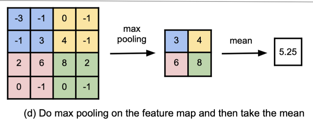
Concept scores: We use Place365 images from test folder as the inputs. Similarly, for each input, we get a $7\times7\times512$ output vector. We need a scalar for each of the scores. To this end, pool max method is used as it can capture both low-level concepts and high-level concepts. More specifically, we take the max pooling on the feature map, and then take the mean to reduce a tensor from $7\times7\times512$ to a $512$-dimensional vector. Figure below visualizes the calculating concept activation using pool max.
From this, the score for each concept is the value at the corresponding index of the vector. For example, concept airplane has an index of 0, so the score of concept airplane is the value at index 0 of the vector. Similarly, the next concept, let’s say boat, will take the value at index 1 of the vector as the concept score.
The authors show that in the latent space of CW, two concepts are nearly orthogonal, while without CW as in standard neural networks, they are generally not. So, the concepts from CW are purer than those of standard methods.
5.5. Results
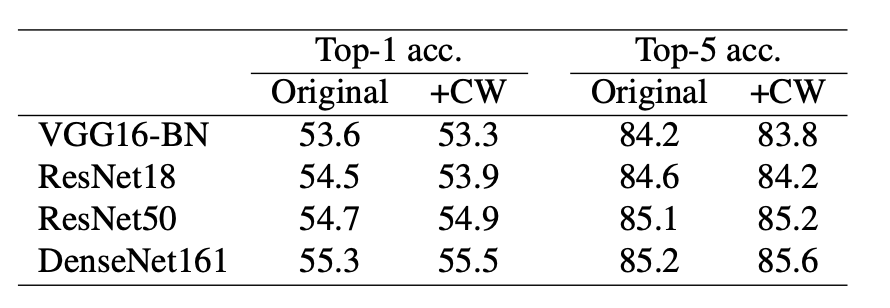
6. Conclusion
Concept Whitening (CW) is a good tool for altering neural network models to make them more explainable. It replaces the batch normalization layer with a CW module to decorrelate the concepts in the latent space. These concepts are transformed into orthogonal vectors where each neuron represents only one concept. As a result, the orthogonal property gains more interpretability power for existing black-box networks.
Some questions remain, such as how we can help the CW to distinguish similar concepts, and how to define the concepts automatically.
Useful links
-
CW source code from the authors